pyroot draw 3d hist ttree python
In this tutorial, you'll exist equipped to make product-quality, presentation-ready Python histogram plots with a range of choices and features.
If you take introductory to intermediate cognition in Python and statistics, then y'all tin can utilize this commodity as a i-stop shop for building and plotting histograms in Python using libraries from its scientific stack, including NumPy, Matplotlib, Pandas, and Seaborn.
A histogram is a corking tool for quickly assessing a probability distribution that is intuitively understood by almost any audience. Python offers a handful of different options for building and plotting histograms. Most people know a histogram by its graphical representation, which is similar to a bar graph:
This article will guide y'all through creating plots like the i above as well equally more circuitous ones. Here's what you'll cover:
- Building histograms in pure Python, without employ of third party libraries
- Constructing histograms with NumPy to summarize the underlying data
- Plotting the resulting histogram with Matplotlib, Pandas, and Seaborn
Histograms in Pure Python
When you are preparing to plot a histogram, it is simplest to not retrieve in terms of bins simply rather to report how many times each value appears (a frequency table). A Python dictionary is well-suited for this task:
>>>
>>> # Need not be sorted, necessarily >>> a = ( 0 , 1 , ane , 1 , 2 , 3 , seven , 7 , 23 ) >>> def count_elements ( seq ) -> dict : ... """Tally elements from `seq`.""" ... hist = {} ... for i in seq : ... hist [ i ] = hist . get ( i , 0 ) + 1 ... return hist >>> counted = count_elements ( a ) >>> counted {0: 1, ane: 3, 2: 1, 3: 1, vii: two, 23: 1} count_elements() returns a dictionary with unique elements from the sequence equally keys and their frequencies (counts) as values. Within the loop over seq, hist[i] = hist.become(i, 0) + ane says, "for each element of the sequence, increment its respective value in hist by one."
In fact, this is precisely what is done by the collections.Counter class from Python'southward standard library, which subclasses a Python dictionary and overrides its .update() method:
>>>
>>> from collections import Counter >>> recounted = Counter ( a ) >>> recounted Counter({0: 1, 1: 3, iii: 1, 2: i, seven: 2, 23: 1}) You tin ostend that your handmade function does virtually the same matter as collections.Counter by testing for equality between the two:
>>>
>>> recounted . items () == counted . items () True It can exist helpful to build simplified functions from scratch as a beginning stride to understanding more complex ones. Let's further reinvent the cycle a bit with an ASCII histogram that takes advantage of Python's output formatting:
def ascii_histogram ( seq ) -> None : """A horizontal frequency-table/histogram plot.""" counted = count_elements ( seq ) for one thousand in sorted ( counted ): print ( ' {0:5d} {one} ' . format ( k , '+' * counted [ k ])) This part creates a sorted frequency plot where counts are represented every bit tallies of plus (+) symbols. Calling sorted() on a lexicon returns a sorted list of its keys, and then you access the corresponding value for each with counted[k]. To meet this in action, you can create a slightly larger dataset with Python's random module:
>>>
>>> # No NumPy ... yet >>> import random >>> random . seed ( 1 ) >>> vals = [ one , three , 4 , 6 , viii , 9 , 10 ] >>> # Each number in `vals` will occur betwixt 5 and 15 times. >>> freq = ( random . randint ( 5 , xv ) for _ in vals ) >>> information = [] >>> for f , v in zip ( freq , vals ): ... data . extend ([ v ] * f ) >>> ascii_histogram ( information ) 1 +++++++ iii ++++++++++++++ iv ++++++ six +++++++++ viii ++++++ nine ++++++++++++ x ++++++++++++ Hither, you're simulating plucking from vals with frequencies given by freq (a generator expression). The resulting sample data repeats each value from vals a certain number of times between 5 and 15.
Building Up From the Base of operations: Histogram Calculations in NumPy
Thus far, yous have been working with what could best be chosen "frequency tables." Just mathematically, a histogram is a mapping of bins (intervals) to frequencies. More than technically, it can be used to gauge the probability density function (PDF) of the underlying variable.
Moving on from the "frequency table" above, a truthful histogram commencement "bins" the range of values and then counts the number of values that fall into each bin. This is what NumPy'south histogram() role does, and information technology is the footing for other functions yous'll see here subsequently in Python libraries such equally Matplotlib and Pandas.
Consider a sample of floats fatigued from the Laplace distribution. This distribution has fatter tails than a normal distribution and has 2 descriptive parameters (location and calibration):
>>>
>>> import numpy equally np >>> # `numpy.random` uses its own PRNG. >>> np . random . seed ( 444 ) >>> np . set_printoptions ( precision = 3 ) >>> d = np . random . laplace ( loc = xv , scale = 3 , size = 500 ) >>> d [: 5 ] array([18.406, eighteen.087, 16.004, xvi.221, vii.358]) In this example, you're working with a continuous distribution, and it wouldn't be very helpful to tally each bladder independently, downward to the umpteenth decimal place. Instead, you lot tin bin or "bucket" the information and count the observations that autumn into each bin. The histogram is the resulting count of values within each bin:
>>>
>>> hist , bin_edges = np . histogram ( d ) >>> hist array([ 1, 0, three, four, four, 10, 13, 9, two, 4]) >>> bin_edges array([ iii.217, 5.199, 7.181, 9.163, xi.145, 13.127, 15.109, 17.091, xix.073, 21.055, 23.037]) This result may not be immediately intuitive. np.histogram() by default uses 10 equally sized bins and returns a tuple of the frequency counts and corresponding bin edges. They are edges in the sense that there will exist one more than bin edge than there are members of the histogram:
>>>
>>> hist . size , bin_edges . size (10, xi) A very condensed breakdown of how the bins are constructed past NumPy looks like this:
>>>
>>> # The leftmost and rightmost bin edges >>> first_edge , last_edge = a . min (), a . max () >>> n_equal_bins = ten # NumPy's default >>> bin_edges = np . linspace ( start = first_edge , stop = last_edge , ... num = n_equal_bins + 1 , endpoint = True ) ... >>> bin_edges assortment([ 0. , two.3, 4.6, half-dozen.9, 9.ii, 11.5, xiii.8, 16.1, eighteen.4, 20.7, 23. ]) The case higher up makes a lot of sense: 10 every bit spaced bins over a peak-to-peak range of 23 means intervals of width 2.3.
From there, the function delegates to either np.bincount() or np.searchsorted(). bincount() itself can be used to finer construct the "frequency tabular array" that yous started off with here, with the distinction that values with zero occurrences are included:
>>>
>>> bcounts = np . bincount ( a ) >>> hist , _ = np . histogram ( a , range = ( 0 , a . max ()), bins = a . max () + 1 ) >>> np . array_equal ( hist , bcounts ) True >>> # Reproducing `collections.Counter` >>> dict ( zip ( np . unique ( a ), bcounts [ bcounts . nonzero ()])) {0: ane, 1: 3, 2: 1, 3: 1, 7: 2, 23: 1} Visualizing Histograms with Matplotlib and Pandas
At present that you've seen how to build a histogram in Python from the ground upwardly, let's see how other Python packages tin do the job for you lot. Matplotlib provides the functionality to visualize Python histograms out of the box with a versatile wrapper around NumPy's histogram():
import matplotlib.pyplot as plt # An "interface" to matplotlib.axes.Axes.hist() method n , bins , patches = plt . hist ( x = d , bins = 'auto' , color = '#0504aa' , alpha = 0.7 , rwidth = 0.85 ) plt . grid ( axis = 'y' , blastoff = 0.75 ) plt . xlabel ( 'Value' ) plt . ylabel ( 'Frequency' ) plt . title ( 'My Very Own Histogram' ) plt . text ( 23 , 45 , r '$\mu=fifteen, b=three$' ) maxfreq = northward . max () # Set up a clean upper y-centrality limit. plt . ylim ( ymax = np . ceil ( maxfreq / 10 ) * 10 if maxfreq % 10 else maxfreq + 10 ) 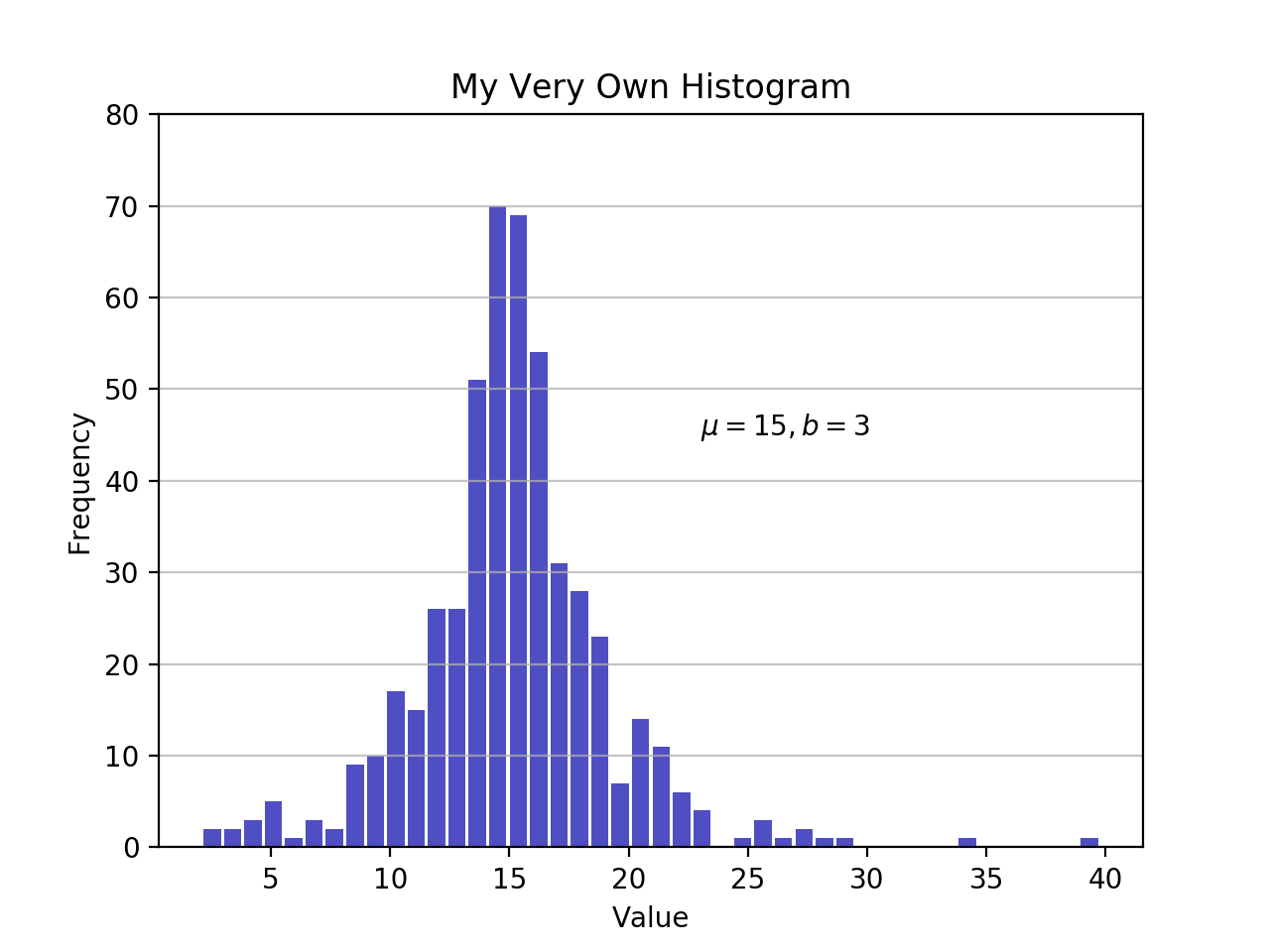
As defined before, a plot of a histogram uses its bin edges on the x-axis and the respective frequencies on the y-axis. In the chart to a higher place, passing bins='auto' chooses between ii algorithms to estimate the "platonic" number of bins. At a high level, the goal of the algorithm is to choose a bin width that generates the most true-blue representation of the information. For more than on this subject area, which tin can become pretty technical, check out Choosing Histogram Bins from the Astropy docs.
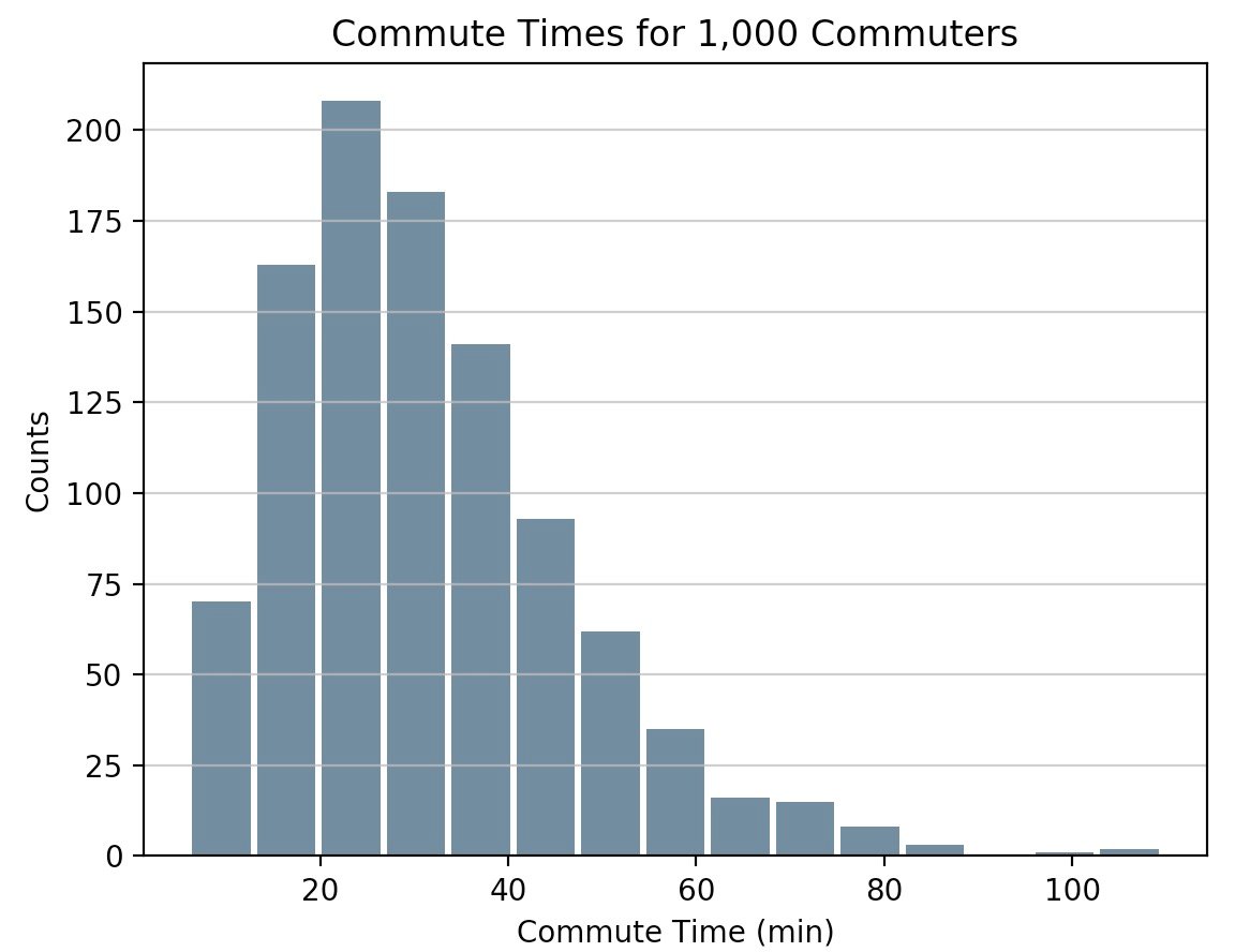
Staying in Python's scientific stack, Pandas' Serial.histogram() uses matplotlib.pyplot.hist() to depict a Matplotlib histogram of the input Series:
import pandas as pd # Generate information on commute times. size , scale = 1000 , ten commutes = pd . Series ( np . random . gamma ( calibration , size = size ) ** 1.5 ) commutes . plot . hist ( grid = True , bins = 20 , rwidth = 0.9 , color = '#607c8e' ) plt . title ( 'Commute Times for 1,000 Commuters' ) plt . xlabel ( 'Counts' ) plt . ylabel ( 'Commute Fourth dimension' ) plt . grid ( axis = 'y' , alpha = 0.75 ) pandas.DataFrame.histogram() is similar but produces a histogram for each column of data in the DataFrame.
Plotting a Kernel Density Estimate (KDE)
In this tutorial, y'all've been working with samples, statistically speaking. Whether the data is discrete or continuous, it's assumed to be derived from a population that has a truthful, verbal distribution described by only a few parameters.
A kernel density interpretation (KDE) is a way to gauge the probability density role (PDF) of the random variable that "underlies" our sample. KDE is a means of data smoothing.
Sticking with the Pandas library, you can create and overlay density plots using plot.kde(), which is available for both Series and DataFrame objects. Merely first, allow's generate two singled-out data samples for comparing:
>>>
>>> # Sample from two different normal distributions >>> means = ten , 20 >>> stdevs = 4 , two >>> dist = pd . DataFrame ( ... np . random . normal ( loc = means , scale = stdevs , size = ( thousand , 2 )), ... columns = [ 'a' , 'b' ]) >>> dist . agg ([ 'min' , 'max' , 'mean' , 'std' ]) . round ( decimals = 2 ) a b min -i.57 12.46 max 25.32 26.44 mean ten.12 19.94 std 3.94 1.94 Now, to plot each histogram on the same Matplotlib axes:
fig , ax = plt . subplots () dist . plot . kde ( ax = ax , legend = Fake , title = 'Histogram: A vs. B' ) dist . plot . hist ( density = True , ax = ax ) ax . set_ylabel ( 'Probability' ) ax . grid ( axis = 'y' ) ax . set_facecolor ( '#d8dcd6' ) 
These methods leverage SciPy'due south gaussian_kde(), which results in a smoother-looking PDF.
If you take a closer look at this function, you lot can come across how well it approximates the "true" PDF for a relatively small sample of 1000 information points. Below, yous can first build the "analytical" distribution with scipy.stats.norm(). This is a class instance that encapsulates the statistical standard normal distribution, its moments, and descriptive functions. Its PDF is "exact" in the sense that it is defined precisely as norm.pdf(10) = exp(-x**2/2) / sqrt(two*pi).
Edifice from there, you can take a random sample of k datapoints from this distribution, then effort to back into an interpretation of the PDF with scipy.stats.gaussian_kde():
from scipy import stats # An object representing the "frozen" analytical distribution # Defaults to the standard normal distribution, North~(0, i) dist = stats . norm () # Draw random samples from the population you lot built above. # This is just a sample, then the mean and std. departure should # exist close to (1, 0). samp = dist . rvs ( size = 1000 ) # `ppf()`: percentage point office (inverse of cdf — percentiles). 10 = np . linspace ( start = stats . norm . ppf ( 0.01 ), stop = stats . norm . ppf ( 0.99 ), num = 250 ) gkde = stats . gaussian_kde ( dataset = samp ) # `gkde.evaluate()` estimates the PDF itself. fig , ax = plt . subplots () ax . plot ( x , dist . pdf ( ten ), linestyle = 'solid' , c = 'red' , lw = 3 , alpha = 0.8 , label = 'Analytical (True) PDF' ) ax . plot ( x , gkde . evaluate ( x ), linestyle = 'dashed' , c = 'blackness' , lw = ii , characterization = 'PDF Estimated via KDE' ) ax . legend ( loc = 'all-time' , frameon = Imitation ) ax . set_title ( 'Belittling vs. Estimated PDF' ) ax . set_ylabel ( 'Probability' ) ax . text ( - 2. , 0.35 , r '$f(x) = \frac{\exp(-10^2/2)}{\sqrt{2*\pi}}$' , fontsize = 12 ) 
This is a bigger chunk of lawmaking, so let's have a second to touch on a few key lines:
- SciPy'southward
statssubpackage lets you create Python objects that represent analytical distributions that you can sample from to create actual information. Sodist = stats.norm()represents a normal continuous random variable, and you lot generate random numbers from it withdist.rvs(). - To evaluate both the belittling PDF and the Gaussian KDE, you need an array
xof quantiles (standard deviations above/beneath the mean, for a normal distribution).stats.gaussian_kde()represents an estimated PDF that yous need to evaluate on an array to produce something visually meaningful in this case. - The terminal line contains some LaTex, which integrates nicely with Matplotlib.
A Fancy Alternative with Seaborn
Let's bring 1 more than Python bundle into the mix. Seaborn has a displot() function that plots the histogram and KDE for a univariate distribution in ane step. Using the NumPy assortment d from ealier:
import seaborn as sns sns . set_style ( 'darkgrid' ) sns . distplot ( d ) 
The call above produces a KDE. There is also optionality to fit a specific distribution to the information. This is different than a KDE and consists of parameter interpretation for generic information and a specified distribution proper noun:
sns . distplot ( d , fit = stats . laplace , kde = Imitation ) 
Again, notation the slight deviation. In the first example, you're estimating some unknown PDF; in the 2nd, you're taking a known distribution and finding what parameters all-time describe information technology given the empirical data.
Other Tools in Pandas
In addition to its plotting tools, Pandas also offers a convenient .value_counts() method that computes a histogram of not-null values to a Pandas Series:
>>>
>>> import pandas as pd >>> data = np . random . option ( np . arange ( 10 ), size = 10000 , ... p = np . linspace ( ane , 11 , x ) / 60 ) >>> due south = pd . Series ( data ) >>> s . value_counts () 9 1831 8 1624 seven 1423 6 1323 five 1089 4 888 3 770 ii 535 1 347 0 170 dtype: int64 >>> s . value_counts ( normalize = Truthful ) . head () 9 0.1831 eight 0.1624 7 0.1423 6 0.1323 5 0.1089 dtype: float64 Elsewhere, pandas.cutting() is a convenient way to bin values into capricious intervals. Permit's say you accept some data on ages of individuals and want to bucket them sensibly:
>>>
>>> ages = pd . Series ( ... [ 1 , 1 , 3 , 5 , 8 , 10 , 12 , 15 , 18 , eighteen , 19 , 20 , 25 , 30 , 40 , 51 , 52 ]) >>> bins = ( 0 , 10 , 13 , xviii , 21 , np . inf ) # The edges >>> labels = ( 'kid' , 'preteen' , 'teen' , 'military_age' , 'adult' ) >>> groups = pd . cut ( ages , bins = bins , labels = labels ) >>> groups . value_counts () kid half dozen adult 5 teen iii military_age 2 preteen 1 dtype: int64 >>> pd . concat (( ages , groups ), centrality = ane ) . rename ( columns = { 0 : 'age' , 1 : 'group' }) historic period group 0 1 kid 1 1 child 2 3 child iii 5 child iv eight child v 10 child half-dozen 12 preteen 7 15 teen eight 18 teen 9 18 teen 10 19 military_age 11 xx military_age 12 25 developed 13 thirty developed 14 forty adult xv 51 adult 16 52 adult What'due south nice is that both of these operations ultimately utilize Cython lawmaking that makes them competitive on speed while maintaining their flexibility.
Alright, So Which Should I Use?
At this point, you lot've seen more a scattering of functions and methods to cull from for plotting a Python histogram. How do they compare? In short, there is no "i-size-fits-all." Here'southward a epitomize of the functions and methods you lot've covered thus far, all of which relate to breaking down and representing distributions in Python:
| You Take/Want To | Consider Using | Notation(s) |
|---|---|---|
| Clean-cutting integer information housed in a data structure such equally a list, tuple, or gear up, and you desire to create a Python histogram without importing any third political party libraries. | collections.Counter() from the Python standard library offers a fast and straightforward style to get frequency counts from a container of data. | This is a frequency table, so it doesn't employ the concept of binning equally a "truthful" histogram does. |
| Big array of data, and you want to compute the "mathematical" histogram that represents bins and the corresponding frequencies. | NumPy's np.histogram() and np.bincount() are useful for computing the histogram values numerically and the corresponding bin edges. | For more, cheque out np.digitize(). |
Tabular data in Pandas' Series or DataFrame object. | Pandas methods such as Series.plot.hist(), DataFrame.plot.hist(), Series.value_counts(), and cutting(), likewise as Serial.plot.kde() and DataFrame.plot.kde(). | Cheque out the Pandas visualization docs for inspiration. |
| Create a highly customizable, fine-tuned plot from any data construction. | pyplot.hist() is a widely used histogram plotting function that uses np.histogram() and is the ground for Pandas' plotting functions. | Matplotlib, and particularly its object-oriented framework, is great for fine-tuning the details of a histogram. This interface tin accept a fleck of fourth dimension to master, but ultimately allows you to exist very precise in how whatever visualization is laid out. |
| Pre-canned design and integration. | Seaborn's distplot(), for combining a histogram and KDE plot or plotting distribution-fitting. | Essentially a "wrapper around a wrapper" that leverages a Matplotlib histogram internally, which in turn utilizes NumPy. |
You tin can also detect the code snippets from this article together in one script at the Real Python materials folio.
With that, good luck creating histograms in the wild. Hopefully one of the tools above will suit your needs. Any you do, just don't use a pie chart.
Source: https://realpython.com/python-histograms/
0 Response to "pyroot draw 3d hist ttree python"
Post a Comment